The emergence of classical neural networks

4 The emergence of classical neural networks

4.1 Early ladder-like nervous system

We begin our examination of the emergence of neural networks in the brain with the early ladder-like nervous systems, as already found in Bilateria. This segmented nervous system was present on both sides of the body and was divided into a sensory and a motor part – a division that is still found today in the neural tube of vertebrates.

· Sensory ganglia: Receptors in each segment generated signals that arrived at the segment’s sensory centre.

· Commissures: From there, the signals were transmitted to the motor side and activated motor function via the motor centre.

· Connections: At the same time, the sensory signals travelled upwards towards the head and reached higher segments. The highest segment received all sensory signals and later developed into the cortex. From there, the signals travelled back down to the segment of origin, where they controlled motor function.

· Motor ganglia: In each segment, motor ganglia formed as intermediate stations along the motor signal pathway. Many neuronal nuclei of the vertebrate nervous system have evolved from these ganglia.

The early bilateral nervous system consisted of two ladder-like systems.

· Crossing nuclei enabled the exchange of signals between the two halves of the body.

· Median nuclei provided control signals for the life-support system.

This system formed the basis for the later nervous system of vertebrates. The following features were retained:

· the division of the neural tube into sensory and motor parts (anterior horn/posterior horn) as well as a lateral horn for the autonomic nervous system,

· the segmentation of the vertebrate body,

· excitatory interneurons, which enabled signal transmission between segments,

· inhibitory interneurons, which created neural competition and ensured that stronger signals could prevail,

· projection neurons, which connected segments to one another and to the developing cortex,

· median neurons in the median nuclei

This meant that all the prerequisites for the emergence of classical neural networks in the nervous system were in place.

4.2 Motor signals in the reticular formation

The reticular formation was an early motor nucleus. Motor signals from one half of the body arrived – like all signals – in the reticular formation. Its projection neurons tap into the signals from the environment with the help of excitatory interneurons or their own dendrites and form signal averages from them. These left the nucleus towards the cortex (we shall not concern ourselves with their further use for the time being).

If the receptive fields of these interneurons are larger, they can combine several motor signals into a single average. The output of such a neuron can be understood, in simplified terms, as a scalar product:

· Each synapse of the interneuron forms a signal unit with an input axon.

· The effect depends on the synaptic strength, which we can interpret as a number between 0 and 1. In AI terminology, this value is referred to as the synaptic weight.

· This value indicates how strongly the synapse transmits the input signal to the averaging neuron.

· The weight of the synapse is multiplied by the firing rate of the signal and represents the contribution of this signal to the total signal.

· The total signal is produced by the additive superposition of all inputs via their synapses.

This component-wise multiplication of weight and input corresponds to the dot product in vector calculus:

Formel

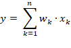
y Output of the neuron

x_k k = 1, 2, …, n Input of the kth synapse

It is tacitly assumed that the weights remain relatively constant after a certain learning phase. The axons of the output neurons left the reticular formation by joining the remaining axons and were able to take on new tasks.

4.3 Hebbian learning: the beginning of the evolution of neural networks

The scalar product describes how the synaptic weights are multiplied by the firing rates of the inputs and then summed. However, these weights are not static – they can change. This is where Hebb’s learning rule comes into play, which is regarded as the first biological learning principle:

· Basic idea: “Neurons that fire together, wire together.”

· Donald O. Hebb (1904–1985): A Canadian psychologist, he formulated the learning rule for neurons in his 1949 book *The Organisation of Behaviour*

· If an input neuron is active at the same time as the output neuron, the synaptic connection between the two is strengthened.

· If an input neuron remains inactive whilst the output neuron fires, the connection weakens.

This creates a dynamic adaptation system:

· Signals that are frequently active together strengthen their synaptic weights.

· Signals that are rarely or never active together lose their influence.

· The neural network begins to recognise and store patterns by adjusting its weights. It develops synaptic plasticity.

From an evolutionary perspective, Hebb’s learning rule was the decisive step:

· A purely feedforward network with fixed connections became a plastic system capable of mapping experiences within its structure.

· This marks the beginning of the development of classical neural networks in the vertebrate brain – and forms the basis for later complex network architectures involving convolution, feedback and specialisation.

Over longer periods of time, as required by Hebbian learning, motor signals exhibit varying frequencies. A single signal corresponds to a muscle; two signals from a joint represent its angle. Multiple combinations of joint angles result in different signal pairs, which, however, do not occur with equal frequency. Hebbian learning reinforces the most frequent patterns: the most frequent signal manifests itself in the weights of an output neuron. If all output neurons of the mean-vector core tap into all input signals, they will, in theory, develop identical weight vectors via Hebbian learning. In doing so, they all document the same body state – the most frequent one, such as a dog standing. Nature had to break this symmetry through neural competition. This is illustrated below.

4.4 Neural competition and breaking of symmetry

The output neurons of the reticular formation began to develop neural competition amongst themselves. Via inhibitory interneurons, each neuron inhibited all the others. This competition knows only one winner: the neuron that first reaches the maximum excitation and triggers an action potential fires first – and, in a ‘ ’, instantly suppresses the weaker excitation of its competitors. The Winner Takes All.

This broke the symmetry: for the most frequent signal, only exactly one output neuron now fired. Since Hebbian learning does not continue indefinitely but is reversed if input is absent for a long time, the remaining output neurons forgot the most frequent signal they had already learnt over time. This made them receptive to the second most frequent signal, at which point learning began anew. This process could be repeated several times. In this way, the output neurons learnt the signals in order of their frequency. The lateral inhibition of the output signals amongst themselves corresponds to the introduction of a non-linearity such as ReLU, without which the network would be unable to develop its ability to distinguish patterns

4.5 Stabilisation through inhibition of the input axons

The output neuron representing the most frequent signal not only sends a recognition signal via its axon but also contacts an inhibitory interneuron. This acts directly on the input axons of the motor signals. Special inhibitory axon terminals dock onto the passing input axons and suppress their activity after they have activated the output neuron.

For this to work, the inhibition of the signal-carrying axons had to begin behind the output neuron that recognised the active signal. This divided the signal pathway for each output neuron into an afferent signal pathway and an efferent signal pathway for the input signals. The inhibition of the input was only permitted in the efferent signal pathway, as the neuron was not allowed to inhibit its own input; otherwise, it would not be able to recognise the stored pattern at all. Since all input axons and also the output axons ran practically parallel to one another, this resulted in a neural network with a bus topology.

This inhibition in the efferent signal pathway is also subject to Hebbian learning:

· The more frequently the most common signal occurs, the stronger the inhibition of its own input axons becomes.

· This prevents the subsequent output neurons of the efferent signal pathway from relearning this signal.

· The most frequent signal remains exclusively linked to a single output neuron.

This finally breaks the symmetry:

· One output neuron permanently represents the most frequent bodily state.

· All other output neurons become free for the next most frequent signals, which they can relearn via Hebbian learning.

· Through Hebbian learning, the output neurons of the reticular formation were able to learn the body’s various motor patterns one after the other in order of their frequency. The more output neurons that were formed in the course of evolution, the more diverse and differentiated the resulting learning map of bodily states became.

· Lateral inhibition could be outsourced from the neural nuclei to a higher-order nucleus, which had to be traversed as the signal ascended to the uppermost segment (cortex).

· The signals ascended from the average nucleus to the cortex and returned from there, as the reticular formation calculates averages from virtually all accessible input signals. In this way, a feedback loop emerged between the cortex and the reticular formation, marking the transition to a deep-layered network. This network combined simple feedforward connections with the ability to represent and store complex patterns – a decisive step in the evolution of neural networks in the vertebrate brain.

We shall refer to the type of step-by-step learning of signals in the order of their statistical frequency presented here as frequency learning.

Deep-layered neural networks may also have emerged in other midbrain nuclei, for example in the limbic system. Unfortunately, the author is unable to provide more precise details on this at present. However, the reticular formation is the most promising candidate, particularly as it was to give rise to the brain’s most important storage system: the cerebellum.

4.6 Summary:

The first deep-layered neural networks with a bus topology emerged in central nuclei because many signals from the entire body were available there. The network’s output neurons were able to utilise this input and, through Hebbian frequency learning and lateral inhibition in the efferent signal pathway, break the symmetry in the network and learn and recognise the existing patterns in the order of their relative frequency. An important mean-value nucleus for this was the reticular formation, from which the network neurons later separated to form independent cerebellar nuclei. Thus, the cerebellar nuclei became the material substrate of the early natural neural networks.

4.7 Hebb’s frequency learning and Sanges’ rule

In 1989, Terrence D. Sanger published the article ‘Optimal Unsupervised Learning in a Single-Layer Linear Feedforward Neural Network’ in the journal *Neural Networks*. He described a neural network with Hebbian learning and lateral inhibition in the efferent signal path, whose learning rule modifies the synaptic weights in such a way that the output units learn the principal components of the input dataset (Principal Component Analysis, PCA). His learning rule extended Oja’s 1982 learning rule, which only stably learns the first principal component. A prerequisite for this learning rule was that the data be centred. Consequently, negative signal components also occur here. This cannot happen in the frequency learning described here, as all firing rates are generally positive as input. Consequently, frequency learning is a form of statistical averaging. For this reason, the frequency learning presented here by the author does not learn the principal components, but rather the signals in order of their frequency. Oja and Sanger were the first to recognise the significance of inhibitory feedback on the input signals and to combine this with Hebbian learning.

4.8 First fundamental theorem for biological neural networks

Biological neural networks first emerged evolutionarily as motor averaging networks in the reticular formation. Their fundamental learning principle was frequency learning, which is based on Hebbian reinforcement and lateral input inhibition and functionally corresponds to Sanger’s rule, but without centring of the input data. , these early averaging networks gave rise to the cerebellar nuclei, which can be regarded as their direct evolutionary descendants.