Human brain theory

19 Mathematical and neuronal image analysis

Created on 27.11.2024

The first applications of artificial intelligence can be traced back to the need to be able to read written text by machine. Bank customers could then have their bank statements filled out at home scanned by an ATM at the bank, which would save them the hassle of typing in the data.

Machine recognition of handwriting requires that an artificial system can first recognise lines. The first step is to scan the written sheet of paper and transfer the brightness of the pixels into numerical values. Then it is necessary to determine in this set of pixels where the brightness changes significantly because there is a light or dark line. To do this, for example, a group of four neighbouring pixels must be examined to see whether the brightness values assigned to them differ to a greater extent. The direction in which the brightness decreases the most can be described as the brightness gradient. This should be determined.

The American Lawrence Roberts developed a method for this back in 1963, which approximately determines the brightness gradient of such a group of four pixels. If you imagine a square mask comprising exactly four points, you can perform the analysis for the entire sheet of paper by first analysing the upper left-hand corner of the sheet, then moving the mask one position to the right and repeating the analysis of the gradient until you have reached the right-hand edge of the image. In this way, the gradient values for the first image line are determined.

You then analyse the second line in the same way, then the third, until you have analysed the last line.

The constant shifting of the mask over the entire image field and the calculation of the gradient for the current four pixels is called convolution in mathematics. If you use the method developed by Lawrence Roberts, you have to perform the convolution twice, which requires two convolution matrices. This is because the gradient is a vector consisting of two vector components that must be determined one after the other by convolution.

The current mask is moved across the image. The image section B it captures consists of four pixels each, which have the following appearance:

 ,

The numerical values f₁ to f₄ represent the image brightness. We choose the symbol f for the image brightness because we want to work with firing rates of the retinal ganglion cells later. The indexing follows the direction of rotation of angles, starting at f_1. And as the rotation of angles in mathematics is anti-clockwise, f₂ is to the left of it, f₃ below it and f₄ to the right of it.

This mask M is convolved with the two Roberts matrices R_x and R_y, which have the following form:

   

and

           ,

where B is the input image and G is the output image. The operator represents the convolution. As two convolutions are performed, the result is a vector with two components that represents the gradient Δ

.

We can also specify the amount of the gradient:

.

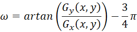
We can also specify the angle ω in which the gradient points:

We calculate the gradient step by step.

.

Further calculations can be made:

so

We will need these results later. They are obtained by applying the Roberts convolution to the first quadruple of points.

We now assume that the image referred to here (i.e. the handwritten sheet of paper) is seen by our eyes and produces the corresponding image on the retina of one eye. The four pixels generated during the electronic scanning of the sheet of paper may correspond to four retinal ganglion cells, which in turn generate the four firing rates f₁ to f₄. Each ganglion cell has (in principle) a receptive field, which is (idealised) circular. Let the four receptive fields of the four ganglion cells be the same size and have the arrangement shown in the following figure.

 

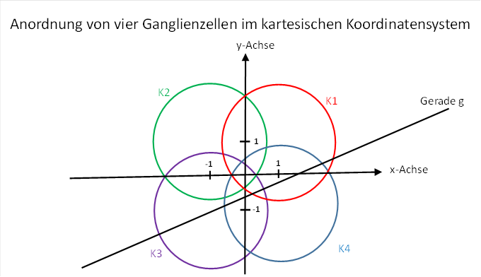
We have already used this illustration in chapter 4.2.2 "The brightness module with lateral signal overlay".

There we had shown that a straight line, when it intersects the four receptive fields K1 to K4 of the ganglion cells, neurally excites these ganglion cells and evokes the firing rates f₁ to f₄:

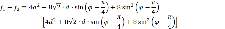
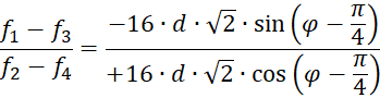
We now calculate some differences somewhat arbitrarily, which we also found when using the Roberts operator.

Now we must note that the angle φ represents the angle of ascent of a straight line in the field of view. The direction of the strongest decrease in brightness is perpendicular to this straight line. Therefore, the gradient will differ from the direction of the straight line by 90°, i.e. by the angle π/2.

The signal evaluation thus provides the gradient α with the help of the receptive fields in the primary visual cortex.

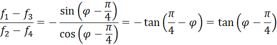
The difference between φ and ω is π/2, as you can easily see:

It can now be seen that the calculation of the angle of rise using the receptive fields of the ganglion cells involved and the calculation of the gradient using the Roberts operator lead to the same result.

Thus, the concept of four overlapping receptive fields , which is intersected by a straight line with the slope φ, provides the slope angle of the straight line, while treating the image with the Roberts convolution operator provides the gradient that is perpendicular to the slope angle.

Since this inclined straight line is called an edge in image processing and the Roberts convolution operator is used for edge detection, the concept of four overlapping receptive fields in conjunction with the non-linear signal attenuation in the primary visual cortex can enable the brain to analyse edges. The Roberts convolution operator fulfils the same purpose, it is used for edge analysis, for which it was ultimately developed.

It is not known whether Lawrence Roberts, when he proposed this operator for image processing in 1963, could have imagined that image evaluation in the primary visual cortex would in principle be carried out exactly according to his principle, but it speaks in favour of his foresight.

In the meantime, many other convolution kernels have been developed that provide better results in image evaluation and image processing.

The Sobel operator, for example, uses a convolution matrix of 9 elements, a matrix of three rows and three columns. It also provides the gradient, but is less susceptible to image noise. The Scharr operator also provides the gradient, but has the advantage of reacting better to symmetry in images.

The mathematical formalism of all these convolution matrices is based on the approximate calculation of the partial derivatives required to determine the gradient. In the transition to the discrete, the differential quotient becomes a difference quotient, so that ultimately differences of function values (here brightnesses) result.

The second derivative of the convolution matrices can also be taken into account to obtain the discrete Laplace operator, which also approximates the image gradient.

It is also possible, for example, to better suppress image noise, change the contrast and make all kinds of changes to photographs, for example, to give them a more pleasing appearance. Gaussian filters are used for this purpose.

Incidentally, no knowledge of the type of neuronal attenuation during signal propagation is required to derive the result!

However, it is worth mentioning that it is not possible to recognise an edge or a line element in an image point without knowing the surroundings of the point. The Roberts operator is based on the (approximate) determination of the increase of the image function in two diagonal directions. However, the slope of a function can always be traced back to the differential quotient, i.e. the derivative. However, the derivative of a function is an environmental property. Therefore, at least four pixels are always required for approximate calculation (in the two-dimensional case of an image).

The fact that the directional sensitivity of the orientation columns in the primary visual cortex can be explained by the overlapping of the receptive fields of the retinal ganglion cells should finally disprove the completely absurd theory that this property of the orientation columns is due to learning. We should get used to the fact that non-linear signal propagation in the brain is the actual cause of many analytical abilities of the vertebrate brain.

Independently of this, there are also learning neuronal networks in the vertebrate brain, but these are supplied with already processed data obtained in the secondary brain system.