Human brain theory

4.2.  Divergence modules with lateral signal propagation 

4.2.1.   The motorised divergence module with lateral signal propagation

 

In motor cortex fields, one observes excitation maxima that wander around when physical movements take place.

In the fac. hbook "Neuroscience" [1] by Eric R. Kandel, James H. Schwartz and Thomas. M. Jessell, Spektrum Akademischer Verlag 1995, chapter 29 presents the research results on voluntary motor activity. It is shown that neurons in the primary motor cortex encode the force and direction of voluntary movements.

In one experimental set-up, monkeys moved a rod with their arm to one of several target points arranged in different directions around a central starting position.

During the movements, the firing rates of very many cortical neurons were measured in the area where the signals from the receptors of the associated muscles and joints arrived.

It turned out that the direction of movement is not encoded by individual neurons, but by populations of neurons. These neuron populations are arranged roughly in a circle around a centre. Depending on the direction of movement, however, only one neuron population is active at a time. Their position relative to the centre codes the direction of movement in such a way that the population vector largely corresponds to the direction of movement.

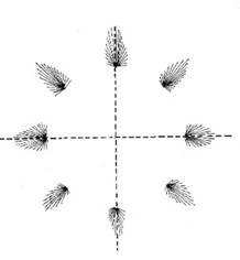
Figure 14: Coding of the direction of movement by active neuron populations

Fig. 12 after [1], page 545, Figure 29.3

 

Is it possible to explain this phenomenon scientifically? Is it possible to deduce the joint angles associated with the movement from the position of such an excitation maximum? Can one perhaps calculate these joint angles from the determined excitation position, i.e. establish a direct mathematical connection between excitation maximum and joint angle?

Yes, this is possible in principle. The motor divergence module creates the information-theoretical access to this topic.

Let's take the shoulder joint as an example, which enables us to raise and lower the arm forwards, but also to move it back and forth sideways. Simplified, this requires four muscles, two of which form a pair of muscles that work antagonistically to each other. The muscles are controlled by motoneurons whose firing rate determines the degree of contraction.

We assign the firing rates f1 and f3 to the first muscle pair. These muscles act against each other, the adjusted joint angle of the first plane depends on the firing rate ratio. For these two receptor signals we choose the exponential approach according to

        

This is always possible if the following approach is taken:

          

It applies

     

We interpret the quantity fm as the mean rate of fire, it satisfies the equation

We call the size u the original size of the joint. It represents (for example) the joint angle with which we raise or lower the arm forward. The value u = 0 may be reached when the arm is extended straight forward. Positive values of u lead to lifting the arm forward, negative values to lowering it. The value f1 is responsible for raising the arm, while f3 is responsible for lowering it.

We assign the firing rates f2 and f4 to the second muscle pair. Here, too, we choose the exponential approach

        

Here the original quantity v is responsible for the lateral movement of the arm, the firing rate f2 moves the arm to the left, the firing rate f4 to the right. In general, the movements will be composed of their two components, because the joint has two degrees of freedom.

We can represent the two original quantities u and v in the Cartesian coordinate system.

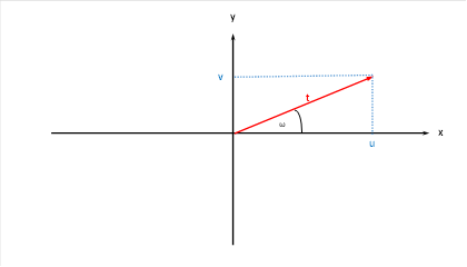
Figure 15: Original quantities u and v in the Cartesian coordinate system

Here the following applies

We call the angle ω the phase angle and t the radius vector in the primal size diagram.

The four firing rates f1 to f4 each reach four neurons of class 3 and 4 via the axons of the generating receptors in the neural tube. The neurons of class 4 project headwards, whereby the firing rate may remain unchanged, so that the (sensory) cortex is reached with the interposition of further neurons of class 4. There, four neurons of class 4 are excited with these four firing rates f1 to f4. Along the entire projection path, the firing rates f1 to f4 may remain unchanged.

We now have to decide which neuron layer receives the input, where the interneurons must be located and which layer is the output layer. We assume that layer four is the input layer. This layer also contains all the interneurons that are involved in signal propagation in layer four.

In this subchapter, we consider the special case of using outpouch layer 3. We assume - as far as evolution is concerned - the very early case that the output layer is a very thin layer. The input neurons of the neighbouring layer 4 may have larger distances to each other. This means that this layer - and with it all other layers - expand in area. This increases the brain size of the associated cortex areas.

Later, in a following chapter, we will lift this restriction and analyse which effects a thickness growth of the outpour layer 3 has.

Two can be considered as outpu layers - layer 3 projects the output to the motor centre (to the motor cortex), layer 6 projects to the median nuclei and layer 2 to the contralateral side. We assume that layer 3 does the real work in this module. Its output is forwarded via pyramidal cells of layers 2 and 6 respectively to the subsequent evaluation units.

In a linear divergence module, the excitations of two neurons overlapped. In a plane divergence module, the spread of excitation occurs in the area where both the input neurons and the output neurons are distributed.

We compare both divergence modules in the following figure.

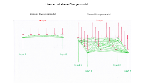
Figure 16: Linear and plane divergence modulus in comparison

Let the plane divergence module have four input neurons. We arrange the four input neurons N1 to N4 in a coordinate system as shown in the following figure.

 

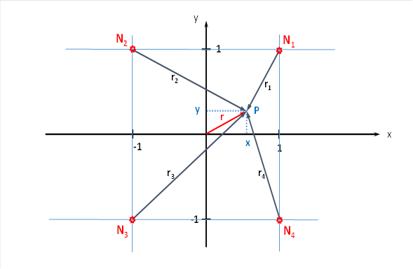
Figure 17: Plane divergence module with four input neurons

The radius vector r as well as the phase angle α and the quantities x and y are linked by the following equations.

.

Let α be the angle that the radius vector r forms with the x-axis.

At the point P with the coordinates P = (x; y), to which the radius vector r belongs, there may now be exactly that neuron which has the greatest excitation among all the neurons in the given square. For this to happen, the joint position must be in a very specific position. We now try to determine the values u and v of the two primal variables from the coordinates x and y of this global maximum.

We assume that the neuronal excitation spreads from the four input neurons in all directions and assumes its absolute maximum in the point P(x; y) with coordinates x and y. That there is such a maximum has already been proven theoretically (see remarks on the Hessian matrix).

From the extreme value conditions to be fulfilled, we determine the values of the necessary primal variables u and v.

For the radius vectors r1 to r4 involved, the following equations are obtained via the Pythagorean theorem:

We consider the following relationships

.

Now we substitute the sum and difference of x and y in the above equations as follows

                  

And thus obtain

If the four input neurons are located in the points , ,  and  and receive excitations with firing rates f1, f2, f3 and f4, then under our conditions the firing rate f of the output neuron at point  can be calculated as the sum of the four excitations involved:

.

If we insert the relationships derived for the four radius vectors r1 to r4 and summarise the common factors, we obtain the following:

For the firing rates f1 and we already chose the exponential approach according to

                                                   

Here, the original size u describes, for example, the joint angle when lifting the arm forward.

Similarly, for the two remaining firing rates f2 and f4, which control the lateral movement of the arm, we chose the default

                                                     

If we insert the above firing rates, the excitation of an output neuron at the point P(x,y) yields the functional equation

The use of the hyperbolic function                      

provides the simplification

Now we apply the following addition theorem for hyperbolic functions

                                   

and receive

About

                

Applies now

 

This excitation function has a global maximum because its Hessian matrix is negative definite in the superposition region of the original functions f1 to f4.

At the point of maximum, the partial derivatives to x and y disappear. Therefore, we calculate these derivatives and set them equal to zero.

We only examine the factor F2

Only the factor F2 can become equal to zero, because the mean firing rate fm is greater than zero, the longitudinal constant λ as well, the function cosh(x) is always positive and also the exponential function is always greater than zero.

Therefore, zeroing the partial derivative with respect to x results in the extreme value condition

Solving for x gives the equation

For u + v we derive a similar formula by setting the partial derivative with respect to y equal to zero.

with

The derivative with respect to y can only become zero when F3 becomes zero.

This results analogously in the zero condition

.

-v once add and once subtract, we arrive at the governing equations for u and v.

We have thus obtained the conditions for the parameters u and v that ensure that the excitation function f(x;y) assumes a global maximum at the point P(x;y) of the cortex.

Indirectly we have also obtained a requirement for the variables x and y. The function artanh is only defined for values in the interval from -1 to +1. x and y must fulfil this condition.

Now we should get an overview of the derived results. We remember the diagram of the original quantities u and v. Here the radius vector t and the angle ω were assigned. We can calculate this angle. We remember:

Substituting v and u gives the equation

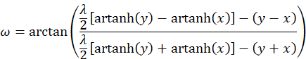
A simpler formula for the phase angle ω results if we express u and v by the radius t and the phase angle. Then for the sum and the difference of u and v the relation applies

Then also

About

Therefore applies

Converted, the phase angle ω is given by the simpler equation

For small values, the function artanh(x) is approximately equal to x.

Therefore, for small x and y the approximation also applies

Expressing x and y by the radius vector r and the angle α gives the following:

      for |x| << 1

Between the phase angle ω to the radius vector t of the two primal quantities u and v and the phase angle α from the radius vector r in the cortical divergence area there is thus a phase shift of π/4 for small values of x and y, here the angle ω lags the angle α by about 45 degrees.

The pointer r, which points to the current excitation maximum of the cortical excitation function, is shifted by π/4, i.e. 45 degrees, against the phase angle ω of the original quantities when the values x and y are small. If the vector t rotates, the vector r also rotates, both in the same sense of rotation, but slightly shifted by about 45 degrees. The original quantity pointer lags behind the pointer r by about 45 degrees.

Now it becomes clear why a maximally excited neuron population rotates around a centre when the monkey also rotates around a centre with its hand.

The identity

substituting the equations for the sum and the difference of u and v gives the equation

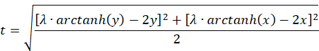
We check what an approximation looks like for small values of x and y, where the function artanh(x) is approximately equal to x.

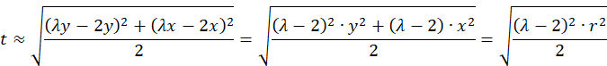
                for small r, i.e. for small x and small y.

Especially with the value

the approximation formula applies for small r

The two radius vectors t and r are for the value   and small values of r and t are approximately equal, moreover they then form the angle of π/4 (i.e. 45 degrees) to each other, the radius vector t runs behind the radius vector r shifted by 45 degrees.

At the end, we want to graphically represent the radius vector t and the phase angle ω as a function of the quantities x and y in diagrams. Remember: x and y are the coordinates of the extreme value, the excitation maximum in the x-y plane, while t and ω describe the primal quantities u and v in polar coordinates.

 

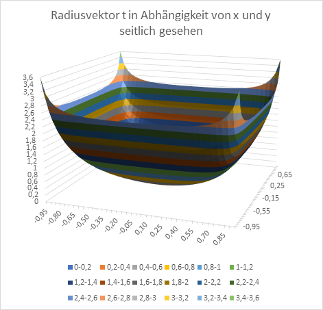
Figure 18: Radius vector t as a function of x and y - seen from the side

 

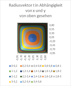
Figure 19: Radius vector t as a function of x and y - seen from above

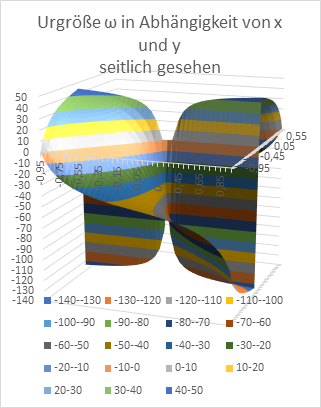
Figure 20: Original size w as a function of x and y - seen from the side

 

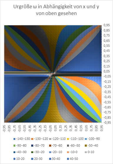
Figure 21: Original size w as a function of x and y - seen from above

 

The above diagram is strongly reminiscent of the representations of the orientation columns in the primary visual cortex. This is because a divergence module is also used there. However, instead of muscle tensions, visually assessable primal variables are used. The principle, however, remains the same.

Mathematicians will be somewhat surprised. They calculate the position of an extreme value depending on the parameters of a function. We go the other way round. From the position of the extreme value, we calculate the parameters originally belonging to it, e.g. the joint angles or the associated firing rates of the muscle tension sensors. Because we want to know what the cortical excitation maxima in the primary cortex fields mean.

The primary cortex areas (they correspond to the sensory centres of the old rope ladder nervous system) project to the motor cortex (which correspond to the motor centres) - without changing the firing rate. The projection axons that do this also do not mix, but transfer the topology to the target areas.

This is why neurologists measure the movement of maximally excited neuron populations in the motor cortex during motor activities. The output of the sensory side finds its counterpart in the motor side.

And we get an astonishing result. The locations of maximum excitation in the primary motor cortex areas encode the joint angles. We can explain why the excitation maxima move back and forth in the cortex and what they mean in the motor case.

The practical tests confirm this theory. If a monkey moves its arm back and forth in a circle, the excitation maximum in the cortex also moves back and forth in a circle. The experimental measurements confirm this theory of neuronal divergence modules.

From a mathematical point of view, this was also to be expected. If an arm is moved circularly, it performs a periodic movement with the period 2π. Thus, the firing rates of the muscle tension sensors of the muscles involved are also periodic functions with the period 2π. If these neuronal excitations arrive in the cortex, they propagate in the vicinity of the input neurons, overlapping additively. However, the sum of periodic functions is always a periodic function again. Since all partial excitations have period 2π, the total excitation also has period 2π, at every point P(x,y) in the neighborhood. If the neuronal excitation is a strictly concave function of distance as it propagates, the total excitation resulting from additive superposition always has a global maximum in some environment whose position in the x-y plane is also a periodic function with period 2π. The maximum therefore rotates about a fixed point, as shown by the experimental measurements. In the case of superposition of neuronal excitations, however, it should be noted that these are strictly concave only in a certain neighborhood of the input neurons, but outside this neighborhood they are strictly convex. Here the distance of the input neurons is subject to certain conditions, so that in the divergence module a maximum coding of the signal parameters occurs.

Since about one third of the cortex cortex is counted as primary areas, we can use this theory to explain the functioning of one third of the cortex cortex. And this without having studied a single synapse. The scientists of the Human Brain Project in particular may take note of this. They analysed millions of synapses without being able to explain the functioning of the cortex cortex.

The performance of the divergence modules in the brain is applied below to the primary visual cortex areas.

 

3.2.2 The brightness module with lateral signal superimposition

 

So-called orientation columns are observed in the primary visual cortex. Their neurons react particularly sensitively to visual stimuli. If an inclined, dark straight line is shown in the field of vision against a bright background, certain populations of neurons react with a strong increase in firing rate. These populations of neurons are arranged windmill-like around a common centre. Each angle of increase corresponds to a different population with maximum excitation.

Whenever excitation maxima occur, or when they start to move and change their position, alarm bells should ring for mathematicians. Many years ago, I too suspected that this was an extreme value problem. Should my knowledge of integral and differential calculus make it possible to put this phenomenon of visual orientation columns on a scientific footing? Even Professor Günther Porath taught me during my studies in Güstrow more than 50 years ago that mathematics was not an end in itself and that it should fill every mathematician with joy and pride when he was able to open up a new mathematical field of application. Should differential and integral calculus give us access to understanding how the orientation columns in V1 work?

Can the ability to solve extreme value problems also lead us to new insights in the primary visual fields?

The answer is clearly yes. The angular sensitivity of the orientation columns in the primary visual cortex is a result of the action of elementary natural laws. This is proven below and has already been presented in my earlier publications.

It is particularly important that no learning processes are necessary for the development of the angular sensitivity of the orientation columns. You don't need a neural network that has to be fed with millions of data sets and that constantly compares and adjusts the output with some specifications (where do they come from?). This angle sensitivity is not learned, it is simply there as soon as the neuronal circuitry of the associated divergence module is fully mature. In flies, this happens immediately after hatching. The lifespan of a fly would also not be sufficient to programme a neuronal network through experience. Some fly species only live for one day.

And this is the crux of the matter! The brain researchers of the Human Brain Project are apparently interested in finding learning neuronal networks in the cortex. To do this, they are studying the almost infinite number of synaptic connections and remember that the world-famous Nobel Prize winner Eric Kandel was able to demonstrate how changes in synaptic strength lead to learning processes. Thus, it was hoped to expose the emergence of intelligence and thought as the result of learning in neural networks.

Hope is the driving force here. Thus, all available resources of the European Union were put into this goal and lofty plans were drafted. All sceptics - often also highly decorated brain researchers - were more or less coerced into joining this project, as there was now only urgently needed funding if one joined the cause.

However, this put the freedom of research at risk!

What do those responsible for this project want to say when they are asked to discuss the following facts?

1.     The cortex cortex is myelin-free almost everywhere, especially layer 4.

2.     Layer 4 receives input from the receptors in the primary areas.

3.     It passes the input to output neurons whose number exceeds the number of input neurons many times over.

4.     The propagation of input excitation to the output neurons leads to local excitation maxima; only these enable brain researchers to attribute a cause to a certain brain activity (e.g. Broca's centre language).

5.     Excitation maxima require a concave transfer function.

6.     The mathematical modelling of the input by parameters (joint angle, pitch, visual stimuli, ...) makes it possible to apply the theory of extreme value determination and thus derive correlations between parameters and the location of maximum excitation.

7.     The occurrence of these excitation maxima in the primary cortex areas is not a consequence of the action of neuronal networks, but a consequence of signal attenuation during the propagation of excitation in the plane.

8.     At least one third of the cortex areas are primary areas, so that about one third of the brain functions can be explained in this way.

Does one then still insist on a claim to sole representation in the field of brain research?

The brain researchers of this world should stop letting the Human Brain Project walk all over them!

In the following, the angular sensitivity of the visual orientation columns is derived mathematically. A different variant of derivation is chosen than in my previous monograph, but the results are the same.

Parts of the text have been taken partly unchanged from my monograph "Brain Theory of Vertebrates" without marking them as citations. This work is also not a dissertation, so plagiarism hunters should not waste their energy on it.

In the visual cortex V1 of vertebrates, one observes a directional selectivity of the so-called orientation columns. These are groups of neurons that run through all six layers of the visual cortex and form small cylindrical columns. Their activity is selectively sensitive to the angle of inclination of a dark line against a light background. The neurons involved must therefore respond to dark objects, they are therefore of the dark-on type.

The input of the second segment comes from the retina. And already there, from a certain stage of evolution, a neuron group with large dendritic fields has established itself. Their signals arrive in the sensory nucleus of the second segment, which is also called the visual thalamus, and form a layer of magnocellular input there.

Via upward projecting neurons of class 4, these signals reach the sensory centre of the first segment, which is the visual cortex. For already in the thalamus the splitting of the modalities took place, each moved into its own modality ladder of the cord ladder system. The various lobes of the brain emerged from these modality ladders of the first floor. In the occipilallobus, the visual signals ended in the fourth layer of cortex. Thus, the fourth layer of the visual cortex consisted of a lower sublayer that received as input the magnocellular signals from the visual thalamus. These served for light-dark vision.

We first analyse the reaction of a magnocellular retinal ganglion cell of the dark-on type when a dark line is moved from left to right across its receptive field against a bright background with a constant angle of attack. The line is moved virtually parallel to itself. We think of the receptive field of the ganglion cell as represented by a circle. Every dark object in the circle will cause an excitation of the ganglion cell, so will this dark straight line.

 

The light-on ganglion cells are responsible (according to the author) for recognising light lines on a dark background. We focus here on the dark-on cells.

 

Let the straight line intersect the circle representing the receptive field of the cell so that part of it becomes the chord in the circle. The length of this chord will determine the firing rate of the ganglion cell. We assume here that the excitation of the cell increases with the square of the chord length. Later, we may be able to drop this assumption once we have grasped the working principle of the orientation columns. At first, we are only interested in the chord length.

 

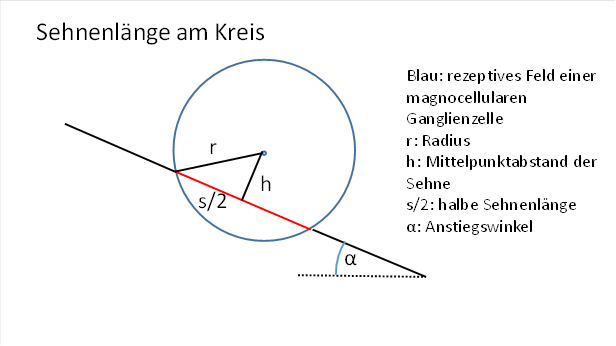
Figure 22: Chord length at the circle

The chord length will depend on the position of the straight line, more precisely on the distance of the straight line to the centre of the circle.

 

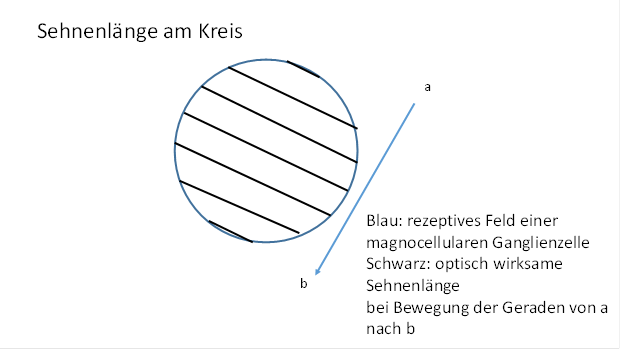
Figure 23: Change in tendon length with parallel displacement to itself

A suitable quantity for calculating the chord length is the distance of the chord from the centre of the circle.

The known radius r forms the hypotenuse of a right triangle whose cathetes are h and half the chord length is s/2. These three quantities are linked via the Pythagorean theorem.

 

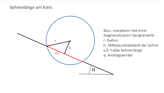
Figure 24: Calculating the chord length on the circle

It is therefore valid:                    (Pythagoras)

This gives the following equation for the square of the chord length:

 

 

In general  apply, since r corresponds to the length of the hypotenuse of a right triangle and h represents the length of a cathetus. Otherwise, the square of the chord length becomes negative, i.e. the chord length becomes an imaginary number. Then the straight line no longer intersects the circle, the formula becomes inapplicable.

 

We assume here that the firing rate f of the ganglion cell in whose receptive field the chord of length s obscures the visual field increases quadratically with chord length. We will neglect a possible proportionality factor here, since it has no effect in extreme value tasks.

 

 

We now consider the chord length or its square using a coordinate system in which the receptive field is not located at the coordinate origin. Let the centre of the circle K, which is to represent the receptive field of the ganglion cell, be the point Pk in the coordinate system, to which we assign the coordinates xm and ym. Then we can also represent the point Pk as Pk(xm; ym).

 

The straight line g, which may intersect the circle K, has the angle of incidence φ to the x-axis. Let its distance from the coordinate origin P(0;0) be d.

 

Let the circle centre Pk(xm; ym) be at a distance rk from the coordinate origin P(0; 0). The straight line connecting both points has the length rk. Let it form the angle φk with the x-axis.

The Pythagorean theorem is mainly used for derivation, as well as the representations of the quantities xm, ym via the sine and cosine of the angle difference. The graphical representation of the relationships necessary for derivation in the following figure is useful.

 

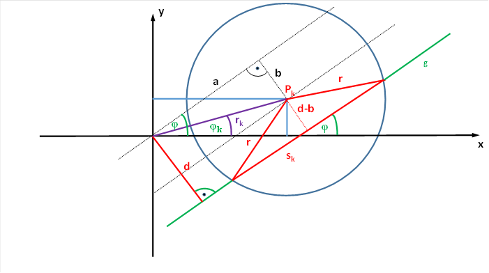
Figure 25: Derivation of the formulas for the chord length of receptive fields

 

The straight line g intersects the x-axis at an angle φ. The centre of the circle is at a distance rk from the origin. The line rk forms an angle φk with the x-axis.

The straight line g that intersects the receptive field of the neuron, i.e. the circle, has the distance d from the coordinate origin. Its distance from the centre of the circle is equal to d-b.

The straight line intersects the circle at two points, creating the chord _sk.

Then we can calculate the length of the half chord using the Pythagorean theorem.

The quantity b is obtained via the sine of the angular difference of the two angles involved.

Thus applies

Substituting this into the equation for half the chord length ultimately yields the equation

We assume (simplistically) that the rate of fire is equal to the square of the chord length _sk.

After deriving a formula for the firing rate of a magnocellular ganglion cell with a large receptive field, we consider four neighbouring retinal ganglion cells. We assign them firing rates f12, f2, f3 and f4 and imagine that their signals may reach the primary visual cortex via the optic nerve and the visual thalamus. Their firing rates may remain unchanged, and their spatial arrangement in relation to each other may also remain unchanged, because the image of the retina in the cortex is true to the topology.

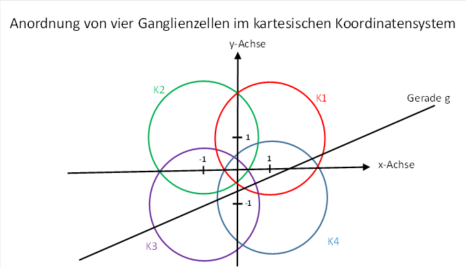
Figure 26: Arrangement of four ganglion cells in the Cartesian coordinate system

 

Each of the four ganglion cells has a circular receptive field with radius rs with respect to the retina. The partial or complete overlap of the four receptive fields is important. The straight line again has the angle of rise φ.

The centres of the four circles should be at a distance of 1 from the x-axis and 1 from the y-axis. Thus they have the distance from the origin of the coordinates .

The following special features apply to this arrangement of ganglion cells:

                             

This simplifies the formulae for the chord lengths s1 to s4 and thus for the firing rates f1 to f4.

           

We simplify.

It applies

Substituting in the fire rates gives the final equations.

The four firing rates f1 to f4 are transmitted via the optic nerve from the ganglion cells to the visual primary cortex and excite four input neurons in the fourth cortex layer. The associated output neurons were located in the directly adjacent layer 3.

But even then, neurons were susceptible to interference, they could fail. It was then advantageous to have replacement neurons nearby that could also receive the signals. The number of output neurons therefore had to grow. The output layer grew in width. The distances between the input neurons increased, because they now had to excite many more output neurons. The reserve neurons, which could compensate for a failure, were already "hardwired", i.e. had all the necessary synapses. Thus, in the event of a neuron failure, a replacement neuron did not have to be formed first.

It is precisely this strategy that led to the emergence of neuron populations that we commonly refer to as orientation columns.

We look at layer S4. It receives the input of the large dark-on neurons of the retina. We focus on the four magnocellular ganglion cells of the retina, whose four receptive fields generate the firing rates f1 to f4 already calculated, depending on the slope of a dark straight line against a light background. These four firing rates arrive - without attenuation - via the thalamus at the myelinated in the primary visual cortex in layer 4. They excite four input neurons N1 to N4 there.

We also represent these symbolically in a coordinate system. Let the previous arrangement of ganglion cells be transferred to the four input neurons N1 to N4.

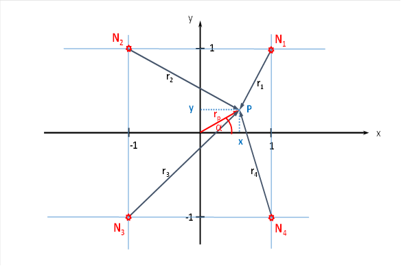
Figure 27: Four cortical output neurons in the brightness module with lateral signal superimposition

The signals arriving in the visual cortex are transmitted from the four input neurons to the innumerable output neurons of layer 5, with the help of the interneurons of layer 4. The propagation is omnidirectional in the plane and satisfies the cable equation for markless fibres. We have to modify this cable equation somewhat because of the excitation propagation in the surface. The square of the distance occurs in the exponent.

We now examine which excitation an output neuron receives at the point P with the coordinates x and y. We call the distance between the origin of the coordinates and the point P the radius vector rp, which forms the angle α with the x-axis. Then we can later express x and y by rp and the sine and cosine of the angle α, respectively.

The output neuron at point P receives an excitation component from each of the four input neurons, the total excitation results from simple addition.

We use the index E at the firing rate f because we want to point out that the excitation propagation is in the plane.

We will call this function the excitation function fE(x,y) of the brightness module with lateral signal propagation.

We will encounter it again in the brightness module with spatial signal propagation.

We assume that the output neuron at point P is part of an orientation column of the visual cortex. At a certain angle of incidence φ of the straight line g, the excitation of this output neuron reaches a maximum. We want to find out under which conditions this occurs.

We must therefore determine when the rate of fire f assumes a maximum. This is the case when the derivative of the function f becomes zero. But according to which quantity do we have to form the derivative?

The output neuron is stationary. It does not move back and forth in the cortex. Therefore, the variables x and y are constant.

In the experiment to determine the directional selectivity of the orientation columns, a straight line was displaced parallel to itself. Thus the angle of attack φ is also a constant. The only variable in the test arrangement is the distance d of the straight line from the coordinate origin. This changes when the straight line is displaced parallel to itself.

So we have to differentiate the function f according to the quantity d and note that all other quantities are constants.

The derivative of a sum is equal to the sum of the derivatives of the individual summands. The exponential quantities are also constants.

We had already derived formulas for the fire rates:

We therefore first calculate the derivatives of the firing rates f1 to f4 with respect to d in order to add them later.

 

We insert these values and set the derivative equal to zero to determine the equation of determination for the presence of a maximum. Since all components are concave functions, a global maximum exists in the common concavity region. By setting the sum of the derivatives to zero, we obtain a conditional equation for the maximum of f.

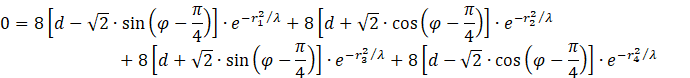
The factor 8 can be divided out. Multiplying out and summing up gives the equation

For the variables r1 to r4 we have already derived the following equations in the last chapter

To shorten the formulas we set

                   

Thus we obtain the extreme value equation

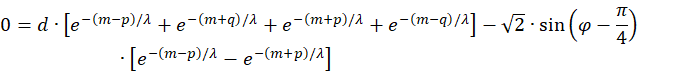
The factor common to all summands  common to all summands can be divided out; it is always greater than zero.

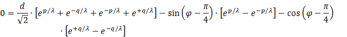
The application of the definition equations

            

Results in

.

We can do without the factor 2.

This equation must be fulfilled so that the neuron fires maximally at point P, i.e. an excitation maximum occurs there. We apply an addition theorem.

This also applies

.

About

Then applies

We apply the following addition theorems for sine and cosine sums

                          

 

Now we can apply a well-known addition theorem for angular functions.

 

Then we get a new equation

We resolve according to the angle φ.

The straight line must have this angle φ so that the firing rate of the output neuron assumes a maximum at the point P(x,y) if the distance of the straight line from the coordinate origin has the value d.

With this, we have finally determined the angle φ at which the cortical output neuron at point P assumes a global excitation maximum.

We see that this angle is a periodic function of the neuron coordinates x and y and also depends on the zero point distance of the inclined straight line with the angle of attack φ.

We can approximate this dependency for small values of x and y.

Because of tanh(x) ≈ x for small x the approximation applies

 

We find the quantities rp and α in the coordinate representation of the visual cortex. Further transformation results in the following representation for the approximation formula (for small y and y)

About

Also applies

           

Therefore, for the approximation formula for small x, y and thus also rp the simplification applies

However, since

the approximation formula for small rp takes the following form:

 

For small x, y and rp, there is a phase shift of 1-π/2, i.e. -32 degrees, between the angle of attack φ of the inclined straight line in the visual field and the radius vector rp in the visual cortex field.

Finally, we want to graphically analyse the relationship between x, y and the angle of attack φ for the case where the output neuron in question is maximally excited. This is different for changing x and y in each case. This can be easily seen in a two-dimensional Excel diagram.

The original formula was:

It is important to point out that the function arcsin(x) is only defined for values with |x|<1. This is only fulfilled if the inclined straight line actually intersects the circles K1 to K4. Only then is the chord length a real number. If the straight line does not intersect the circles, there are also no firing rates; the four magnocellular ganglion cells involved in the retina then deliver no signal to the cortex. The formula for the angle of attack φ of the inclined straight line is then not applicable.

In the following we show the x-y-diagram, which was generated with Excel. Here, the value d = 0.1 was used as the zero point distance of the inclined straight lines. In order for the excitation to assume the maximum value at point x and y, the angle of attack φ of the straight line must assume the values shown in the diagram (in radians).

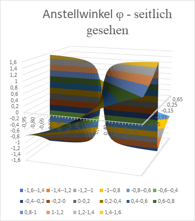
Figure 28: Angle of attack Phi of a straight line as a function of x and y - seen from the side

 

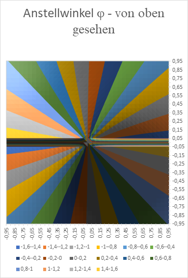
Figure 29: Angle of attack Phi in the brightness module with lateral signal superimposition - seen from above

We see the typical windmill-like arrangement of the neuron populations for the different angles of attack φ of the straight lines.

Incidentally, lateral neighbour inhibition, in conjunction with the "race of the action potentials", leads to the fact that only output neurons in the immediate vicinity of the excitation maximum are excited. These neurons reach their action potential fastest, so they are the first to fire. Their action potential destroys the excitation of all neurons in the surrounding area, since these neurons have not yet been able to reach the excitation threshold for triggering an action potential. The neurologist says to this: The Winner Takes all it. The winner takes it all!

This early primordial state of the magnocellular visual system was altered by a thickness growth of layer 3. Prior to this, the magnocellular ganglion cells of the light-on type developed. The light-on type was signal-compatible with the dark-on type.

This meant that the outpour layer of the dark-on type could also be supplied by the input from the overlying layer 4-light-on. As an effect, the formation of orientation columns now occurred, which did not only react to black or white lines, but to lines with any grey value in front of a grey background with a different grey value.

Just as with the colour module with vertical signal propagation, the emergence of a new modality now took place when the outpu layers of the cortex cortex also expanded in area. We call this new modality the orientation modality of the magnocellular dark-on system. Its output informs the presence of black line elements. In the magnocellular light-on system, a new modality also emerged, the orientation modality of the magnocellular light-on system. It analyses the presence of white line elements.

As all the new modalities became independent and separated in the course of evolution, there were as many retinal images as there were orientation columns after they split. Each retinal image was responsible for an angle and a zero point distance. At the same time, there was a separation into white and black lines. It is roughly as if, instead of one television set, 60 televisions were used, half of which displayed the white line elements and the other half the black ones. Here, each television would only be responsible for those line elements of the original picture whose orientation angle lies in a very specific angle interval with a 30 degree interval width. The first television would therefore only display white line elements whose orientation angle lies between 0 degrees and 30 degrees. The television next to it would display white line elements whose angle lies between 30 and 60 degrees. Each neighbouring TV would increase the preferred angle interval by another 30 degrees, so there would be 30 TVs for the white line elements. The remaining 30 televisions would have the same selection for black line elements.

It must be remembered here that the middle cell column, i.e. the orientation column with the coordinates x = 0 and y = 0 was there first and detected the modality white or black. Its output occupied a separate area in the secondary cortex.

As a result, the animals that produced this conquered a new living world. They could now recognise shapes in the twilight, even if the weak moonlight did not allow colour recognition.

Later, when the outpouch layers of the colour modules also gained thickness, these animals could also recognise shapes that were coloured during the day.

Thus, brightness vision and also colour vision developed into form vision. Orientation columns could recognise the angle of attack of a straight line in the field of vision if it had any shade of grey or colour. Both the angle of attack and the shade of grey or colour were detected, both in parallel and simultaneously.

The most beautiful thing about it was that this did not have to be learned. As soon as the neurons in the brain were fully mature in the relevant layers, this performance could be achieved.

In contrast, creatures in which cortical maturation does not occur until after birth still have to go through the maturation phase before they can recognise contours of grey or coloured objects.