Human brain theory

4.  Divergent modules of the brain 

In a divergence module, signals of different origins are superimposed. They arrive in different input layers, between which there are output layers. Signal attenuation leads to extreme value coding of the output. How did this happen?

The last important step on the path of the vertebrate brain towards the primate brain also took place gradually and began insidiously in early prehistoric times.

Neurons were prone to malfunction, they could malfunction for many reasons or even die. It was therefore advantageous if signals were transmitted via several parallel signal paths. Two neurons whose axons transmitted the same signal doubled the signal reliability.

If one distributed a signal to several neurons at once, then the reliability increased further. Then even several neurons could fail without depriving the body of an important function.

Of course, in the target structure that was to receive this signal, the signal divergence had to be reversed. Thus, in many structures we find large, magnocellular neurons with a large dendrite tree that receive the signal previously distributed to several or many axons again and reverse the signal divergence. We find such convergent neurons in the magnocellular part of the nucleus ruber or as Betz pyramidal cells in the cortex, as well as in the striatum, where they form the striosomes. Thus, the signal divergence could be reversed by convergence neurons.

In the course of evolution, where sufficient space was available or where it could be easily created, redundant signal transmission became the standard. Already in the neural tube, a signal is often distributed to several neurons.

One neuron nucleus in the human brain, the olivary nucleus, has a particularly strong signal divergence. Here, each input signal is distributed to a very large number of output neurons. As a result, this nucleus becomes extremely inflated.

As its output reaches the cerebellum, the number of Purkinje cells there also grows almost immeasurably. The cerebellum cortex expands extremely. Due to lack of space, the surface becomes wrinkled so that it can expand even further.

But the cortex and all its cortex lobes also show this signal divergence. The number of cortical input neurons is extremely small in relation to the cortical output neurons.

The level of evolutionary stage of a species can be clearly related to the increase in size of the nucleus olivaris, cerebellum and cortex, which is predominantly, but not exclusively, due to signal divergence.

This tendency takes on an extreme degree in the human cortex. Thus, even the cortex surface is folded to accommodate the maximum number of output neurons in the available volume.

Here, as the author of this monograph, I must reproach the supporters and planners of the Human Brain Project for not at all getting to the bottom of the question of the reason for this enormous increase in the number of neurons in the olivary nucleus, the cerebellum and the cortex (and other structures) and also for neglecting the consequences of this development.

These researchers established the unproven dogma that intelligence and thinking, as well as the entire functioning of the brain, could be explained solely by studying synaptic connections. So far, no proof of the correctness of this dogma has been provided.

It is like claiming that the laws of heat propagation along a copper wire can be discovered by studying the velocity of the individual copper atoms, so the velocity of each atom must first be determined exactly.

Of course, the temperature of a copper wire depends on the speed of the copper atoms, which is called Brownian motion, but the result is a statistical one. The mean value of the speed of the atomic movements gives the temperature. Statistically, one can abstract from the concrete atom, and atoms no longer appear in the formulas for temperature distribution.

And the temperature distribution along the copper wire also additionally depends on the distance to the heat source. Here it requires the solution of a differential equation taking into account the boundary values.

Why do I come up with this simple example of heat propagation in a copper wire?

Because there is possibly a great analogy between the propagation of heat in substances and the propagation of a neuronal excitation.

If one imagines the propagation of excitation in the same way as the propagation of sound, heat or electrical charges in the form of ion clouds, one abstracts from the existence of atoms, molecules or even neurons. One only considers the location of the signal input, the location of the signal reception and the distance between the two. One assumes a distance-dependent damping of the sound intensity, the heat transfer or the neuronal excitation. Now one determines the transmission parameters in the theoretically derived formulas and confirms them experimentally.

Neurons are superfluous in this model.

It is unacceptable that the experts of the Human Brain Project, especially the mathematicians and physicists among them, simply ignore simple natural laws that apply to the propagation of neuronal excitations, even though they can now be found even in Wikipedia (which is often disparagingly rated among scientists). Thus, in the German Wikipedia, under the search term "action potential", one finds the remarkable sentence:

"In 1952, Alan Lloyd Hodgkin and Andrew Fielding Huxley presented a mathematical model [9] that explained the emergence of the action potential in the giant axon of the octopus through the interplay of various ion channels and became famous under the name Hodgkin-Huxley model . For this discovery, the two researchers, together with John Eccles, received the Nobel Prize for Medicine in 1963."

Likewise, in Wikipedia you can find the complete derivation of the cable equation for excitation propagation on unmyelinated axons.

All neuroscientists are familiar with the fact that the cerebral cortex belongs to the so-called grey matter and the axons running in it are (mostly) not surrounded by any myelin layer. There are exceptions in some areas of the visual cortex, where macroscopically recognisable white stripes occur within the grey matter (Gennari stripes or Vicq-d'Azyr stripes). This is why this cortex area is also called area striata (German: gestreifter Bereich). Apparently, important information is transmitted here via fast-conducting, myelinated axons into neighbouring cortex fields. This information must have to do with motion detection because it must reach its evaluation areas promptly.

The existence of grey matter in the cortex, together with the natural laws of neuronal excitation propagation, in particular the cable equation for markless fibres, gives us the crucial clues to scientifically analyse signal processing in the cortex cortex and in all other nuclei with markless neurons.

In this respect, the researchers involved in the Human Brain Project and especially the coordinators and planners responsible for this project must be reproached for negligently or even deliberately disregarding or even trampling on valid laws of nature. The complete lack of any reaction to my previous publications in my monograph "Brain Theory of Vertebrates for the Human Brain Project of the European Union" shows the ignorance of those responsible.

The cable equation for the propagation of neuronal excitations along an axon gives us the direction for a new view. It turns out that only the distance of the target site from the site of signal input counts. The vast numbers of neuronal synapses involved in signal propagation, which can number in the tens of thousands or hundreds of thousands, are in principle irrelevant!

If a neuronal excitation propagates along an axon whose diameter is assumed to be constant, then the following equation applies to the excitation at a distance r from the start of the axon

,

where λ is the so-called longitudinal constant of the neuron. The indes l in E_l indicates that linear propagation along an axon is present here.

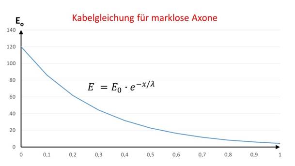
Figure 6: Cable equation for markless fibres

Often, however, the excitation spreads over the area. A cortical input neuron excites a multitude of output neurons in the immediate or distant surroundings in the cortex area. To do this, it either forms a widely ramified dendrite tree or uses interneurons for signal distribution in the area. Here again, almost innumerable synapses are involved, but these can be completely neglected because only the distance from the feed-in point and the longitudinal constant of the input neuron enter into the equation here. This is permissible because the cortex cortex counts as grey matter.

In this case, the cable equation must be specified for an excitation propagation in the plane, in the negative exponent, instead of the distance r, the square r² of the radius of the circle, in whose area the output neurons are located, enters.

with

.

The reason is that the ion cloud, which is ultimately responsible for the potential difference between the cell interior and the extracellular space, does not spread linearly along a single axon, but distributes itself in the plane. Of course, this requires axons, but these branch extremely and thus supply the target neurons in the surrounding area.

And it is of course questionable whether the cable equation for markless fibres can be applied in its previous form to the cortex. Its experimental verification was originally carried out on the giant axon of the squid. The axons of the neurons and interneurons in the cortex, but also in other grey nuclei, are much thinner, much more branched and sometimes have a spatial extension. Therefore, in my monographs, I have assumed an exponential attenuation for these types of neurons, which depends quadratically on the distance. This type of excitation propagation is shown symbolically in the following diagram.

 

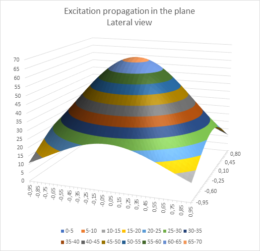
Figure 7: Excitation propagation in the plane - seen from the side

 

Seen from above, the following view emerges:

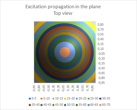
Figure 8: Excitation propagation in the plane - seen from above

Often the neuronal excitation spreads out in space - after all, the cortex layers are not infinitely thin. In this case, one could assume that the radius would enter the cable equation with the third power:

.

I have rejected such an approach. For this to happen, the number of axome branches would have to approach infinity and be distributed quasi continuously in space.

However, this is not so. It is easier to imagine that one first imagines that the axons branch out in the plane like a tree. Here, a quadratic dependence would be expected, since the excitation is distributed approximately in the plane.

Then imagine that the existing axons could simply be bent in such a way that they would branch out spatially in a tree-like manner. The bending would not change their transmission characteristic.

This gives us a new formula for neuronal excitation for propagation in the plane and in space.

It is certainly easy to imagine that the firing rate f of a neuron, which is located at the position x or at the distance r from the signal supplier and receives its excitation f₀ under consideration of a signal attenuation, also depends on this distance. Here, too, the distance enters the formula with the second power, and instead of the input excitation E, the firing rate f of this signal supplier is given.

Then, as a first approximation, the following applies to the rate of fire f

     

The following equation applies for the radius r in the plane

.

In space, the following equation applies to the radius r

.

Generally, not a single input neuron will conduct its excitation to the cortex or into another structure, but there are always several neighbouring input neurons in the cortex that are active. Then the excitation fields of the different input neurons overlap additively, a sum excitation results.

Now, one cannot simply use the cable equation of the Hodgkin-Huxley model

 

                  (Hodgkin-Huxley model)

 

by the equation

 

                (used in this monograph)

 

because they are considered more suitable for cortical neurons from a physical point of view. There must be other solid reasons for this.

 

One solid reason is the occurrence of maximum values of neuronal excitation that move around when examination parameters change. When superimposing neuronal excitations, variable maximum values cannot occur when applying the Hodgkin-Huxley equation. Only spatially variable minima are possible.

 

We discuss excitation propagation and the emergence of excitation maxima from a mathematical point of view.

In this monograph, we restrict ourselves to the case of excitation propagation in a plane; this corresponds approximately to excitation propagation in a relatively thin neuronal layer in the cortex cortex. The input neurons are located in the fourth cortex layer, here the neuronal excitation spreads (simplified) in the plane.

The excitation function is strictly concave in a certain circle around the input neuron and has a maximum at the location of the input neuron. This is shown by the calculation of the Hessian matrix.

The starting point is the excitation function f with the function equation for the plane. The function f is twice continuously differentiable.

The Hessian matrix H is defined by the second partial derivatives:

.

The calculation of the partial derivatives yields the Hessian matrix:

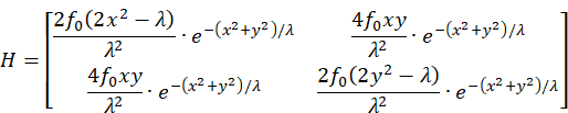
The Hessian matrix is negative definite and the function f strictly concave if all even principal minors are greater than zero, but all odd principal minors are less than zero.

The first skin minor is equal to f_xx and is negative exactly when the condition

is fulfilled. This is true for all values x that satisfy the inequality

fulfil.

The second principal minor of the Hessian matrix is equal to H and must be greater than zero. Therefore the equation

be fulfilled. This means

.

Considering the fact that the longitudinal constant λ > 0, the firing rate factor f_o > 0, and the exponential function is likewise always greater than zero, the only remaining condition is

.

This is in compliance with

is fulfilled exactly when the inequality

is fulfilled.

Then the first inequality is also automatically fulfilled.

Thus the excitation function

is strictly convex if the radius vector r satisfies the condition

is fulfilled. Within the circle with this radius r, this function is strictly convex and has the only global maximum within this circle.

A shift of the function to another point leads to the shift of the circle in which the shifted function is strictly concave. This means the following:

The shifted function

Is strictly concave and has a global maximum in the area that satisfies the condition

suffices.

Every input neuron located at the point x₀ and y₀ with the firing rate f₀ has exactly this strictly concave excitation function.

An additive superposition of the excitations of m input neurons N , N₁₂ , ..., N_m , which are located respectively at the points P₁ (x ;y ), P₁₁₂₂ ; (xy₂ ), ..., P_m (x ;y_mm ), leads to the following equation for the total excitation function f:

 

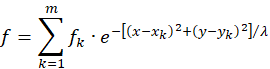
If such excitation functions f_k , which are arranged at different points in the coordinate system, overlap, whereby the circles in which they are strictly concave also overlap, then the existence of a common global maximum in this overlay area is assured. For sufficiently large values of λ (for example, for λ = 9), any number of superpositions of such excitation functions always possess exactly one global maximum if the signal-providing input neurons are distributed arbitrarily in a square with side length 2, if the origin of the square lies in the coordinate origin and the square sides are aligned parallel to the coordinate axes, for example. The strict convexity of such a superposition then results automatically.

The only parameters that occur in the total excitation f are the firing rates f₁ , f₂ , ..., f_m of the m input neurons These can be, for example, the signals of muscle spindles of a joint, as well as the signals of the associated tendon receptors, but also the signals of neighbouring magnocellular visual projection neurons. Almost every modality can send its signals into such divergence modules. Such divergence circuits are clearly recognisable by the fact that the number of input neurons is significantly smaller compared to the number of output neurons. Another feature is the occurrence of excitation maxima that wander around as the input firing rates change.

A note on the orientation columns in the primary visual cortex. They react selectively to the angle of attack of an inclined straight line. A neuron in such an orientation column reacts with maximum excitation when the angle of attack of the straight line assumes a certain value φ. At other angles, the excitation decreases. It is completely incomprehensible to me how one tries to explain this behaviour of the neuron via learning processes in neuronal networks. Why go to such lengths when a simple solution is obvious? A solution that uses simple laws of periodic functions and their linear combinations.

If a dark straight line intersects the circular receptive field of a magnocellular ganglion cell that responds to dark objects, the firing rate of this cell is a strictly monotonic function of the chord length.

If the straight line rotates around a point within the receptive field, the chord length and thus also the rate of fire is a periodic function of the angle of attack φ of the straight line. The period of this function is equal to π.

If four such ganglion cells with circular receptive fields are arranged in such a way that their receptive fields overlap and have a common sub-area, and if a dark straight line rotates around a fixed point in this common area, the firing rate of each ganglion cell is also a periodic function of the angle of attack φ of this straight line. The period is equal to π in all cases.

If these four firing rates arrive in the visual cortex in the corners of a quadrilateral, and any neuron within this quadrilateral receives the neuronal excitation, the resulting firing rate is also a periodic function of the angle of attack φ with the period π when the individual firing rates are additively superimposed.

Every periodic function has extreme values, both minima and maxima.

This is also true if there is distance-dependent damping, because the damping of each excitation contribution is a constant quantity if the location of all neurons involved is invariant.

If the distance-dependent damping takes place through a concave function, there is a global maximum whose position is also a periodic function of the angle of attack φ of the straight line. For exactly one angle of attack φ_max the excitation of the neuron reaches a global maximum.

Thus, the behaviour of the orientation columns in the primary visual cortex is a regularity. The excitation of a (stationary) neuron is a periodic function of the angle of attack.

 

After these explanations, it would actually no longer be necessary to carry out the lengthy calculations that show that orientation columns have exactly the behaviour that has been proven by measurement. Every mathematician would have to agree at this point that the observed behaviour must occur according to law. The observed behaviour of the neurons in orientation columns can also only be explained if the transfer function for neuronal excitations is a concave function of the distance.

After presenting the elementary mathematical basis for divergence modules and the maximum coding of parameters that takes place in them, we can analyse concrete divergence modules of the human brain in more concrete terms.

 

4.1       Divergence modules with vertical signal mixing

4.1.1.  The colour module with vertical signal mixing

 

The following figure is intended to show the structure of a divergence module with vertical signal superimposition in the primary visual cortex. We select only the colour system red-green as an example. The layer thickness S4 of the outpu layer S4-green has already increased, its output neurons are signal compatible with both the input signals of the green receptors and those of the red receptors. Therefore, each output neuron receives input from below as well as above.

Each pixel of the retina is thus assigned a colour module, assuming that the visual cortex cortex only developed thickness growth. Later, we examine the case where there was width growth, and finally we examine the case where there was both thickness growth and width growth.

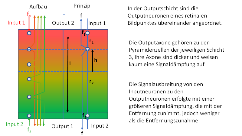
Figure 9: Divergence module for colour vision red-green

The above figure is divided into two parts by a blue line: on the left is its real structure in the cortex, on the right the principle of signal propagation and the quantities required for the mathematical description.

Symbolically represented are the two output neurons belonging to a pixel of the retina with mutually inverse signals f₁ = Red-On/Green-Off and f₂ = Green-On/Red-Off according to the common counter colour theory. We shorten the notation and speak in the following of the green-on neuron and the red-on neuron in a simplified manner.

Exactly on the connecting line of the two input neurons, the output neurons are distributed at about the same distance.

Input and output neurons thus form a narrow eye dominance column.

Let f₁ be the firing rate of the red-on neuron and f₂ be the firing rate of the green-on neuron.

Originally, each class 4 input layer had an associated class 3 output layer just above it - so both the submodalities and the neuron class layers divided and rearranged themselves for each submodality.

This is how the input layers 3-Green-On and 3-Red-On were created.

However, since the red-on receptor was a derivative of the green-on receptor, they were both signal-compatible, i.e. signal-related. Therefore, the output neurons of the lower output layer S3-Green-On could also receive the excitation from the output neurons of the upper layer S4-Red-On. The output layer S3-Red-On became superfluous and regressed in the course of evolution.

The excitation transmitted from the input neurons into the system should propagate through the layer and reach every neuron of the eye dominance column. The specified cable equation for markless axons applies here.

We consider a selected output neuron, which may have the distance r₁ and r₂ from the input neurons. The excitations of both input neurons excite the output neuron according to the formula

The following applies here:

                 

As already shown on the Hessian matrix of the transfer function of a single neuron, there is a global maximum of the firing rate. We want to know where the output neuron with the maximum excitation is located at given firing rates f₁ and f .₂

We determine the maximum by setting the derivative to zero.

We note that the distance between the two input neurons is equal to 1, the output neuron has distance h from the centre of the output layer.

Then applies:

We form the derivative after the variable h and set it equal to zero.

First, we reinsert the quantities r₁ and r₂ and obtain an intermediate result for later use in the convergence grid.

 

 

Equal factors on both sides fall away.

                       (Main formula 1)

We again insert the equations for r₁ and r₂ and obtain

                 (Main formula 2)

 

We logarithmise

 

About

For all values x with |x| < 1.

Because h lies in the interval from - ½ to + ½, as 2h lies in the interval from -1 to +1, we can apply this formula and obtain the relation

   

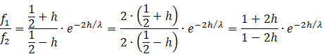
This is equivalent to the equation

               (Main formula 3)

 

The main formulas 1 and 2 allow to calculate the necessary firing rate ratio for an output neuron in the colour module, which takes on the maximum excitation within the whole colour column at the height h.

The function

allows us to examine the firing rate ratio as a function of the height x. We consider that x must be a positive number between 0 and ½, because we have set the total thickness of the colour module equal to 1. For example, the function f has the following appearance for the value λ = 5:

 

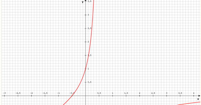
Figure 10: Fire rate ratio in the divergence grid as a function of x

The quantity x in the diagram corresponds to the height h in the divergence module and can assume values between -0.5 and +0.5.

For x = 0 the function has the function value 1, then both firing rates are equal and the maximum neuron is in the middle between both input neurons.

For h = - ½ the function value is zero. In this case f₁ = 0. For h= + ½ the function value becomes infinite. Here f₂ = 0.

Note in the above diagram that only positive function values can occur. Both firing rates are positive, therefore their quotient is also positive.

The described divergence module with vertical signal mixing and the input of the red- and green-sensitive visual receptors produces a maximum-encoded output in the eye dominance column. The maximum excited output neuron encodes the mixing ratio of the colours red and green, for which both visual receptors have different sensitivity curves. If the mixing ratio changes, the excitation maximum moves up or down. Thus, the divergence module in the wavelength range red-green recognises a colour, i.e. also a wavelength.

Three such modules are located one above the other in the cortex, each covering a different wavelength range. Let us call the totality of these three modules the colour module. Then the following statement applies:

The three-part colour module with vertical signal propagation in the visual cortex can recognise colours in the wavelength range red-green-blue and characterise them by a maximum coded output with respect to the wavelength. It can recognise colours.

When the output leaves this colour module (up or down) and there is subsequently a lateral neighbour inhibition between the output signals, only those neurons remain active that are in the immediate vicinity of the excitation maximum. The excitation of the remaining neurons in the entire eye-dominant column falls victim to lateral inhibition. This creates an output vector with sparse coding.

The output of this module can be assigned to a new modality that did not exist in the brain before: colour.

Now began a process that ultimately reached a temporary climax in Homo sapiens. The new modality of colour became independent. As, incidentally, did all the other new modalities that emerged in the various cortical divergence grids.

How do we imagine independence?

It is as if a new type of receptor had emerged that gave rise to this new modality. The output neurons of the divergence lattice took on the role of receptors. Their output moved headwards upwards and established a new ladder segment in the old cord ladder system. Above the old cortical segment, which was actually the last segment in the old cord ladder system, new ladder segments for the new modalities emerged. But since the space upwards was limited by the cranial bone, the newly emerging ladder elements of the newly created modalities simply bent sideways. Thus, the cortex also grew laterally, the lobi underwent a strong lateral expansion and, following the skull bones, bent into half-shells. Lack of space then led to the formation of folds here too. This development is described in more detail in a separate chapter at the end of this book. Thus, in addition to the primary cortex, the secondary cortex developed, which is also called the association cortex and is a sign of higher intelligence.

However, the divergence module with vertical signal overlay was expandable. In the course of evolution, the growth in thickness of the outpouch layers was complemented by growth in width. Species that succeeded in this were able to produce divergence modules in which excitation spread both vertically and horizontally. In the motor cortex, a lawful consequence of this lateral signal divergence was the emergence of joint angle analysis by maximally excited populations of neurons that rotated around a centre during periodic angle change. In the visual cortex, orientation columns emerged whose maximal excitation represented the slope of a straight line in the visual field. Here, the angle of rise of the straight line was analysed by the magnocellular outpouch layer in terms of its brightness (white, greyscale, black), while the parvocellular layers were able to detect the colour of the inclined straight line. This will be explained and proven in the chapter on the divergence modules with spatial signal superposition. But before that, let's look at the brightness module with vertical signal superposition.

It seems necessary to assign the output signals created by the colour module with vertical signal mixing to a new modality: colour.

Initially only mixed colours red-green, later in humans the spectral range from red via yellow and green to blue, there were now neurons whose maximum activity was assigned to a specific colour.

Although the colour module with vertical signal mixing was presented first in this monograph, there was a module with vertical signal mixing that must have been created much earlier. This is because the colour module requires two different types of visual dyes. At first, there was only one, and it enabled light/dark vision. The working principle is the same as for the colour module.

 

4.1.2.  The brightness module with vertical signal mixing

 

The following figure is intended to show the structure of a divergence module with vertical signal superimposition. This module is located below the colour module and processes the output of the magnocellular retinaneurons of the light-on and dark-on type. We assume that the light-on receptors evolved from the dark-on receptors. This is why the evolutionarily younger layer is at the top, as is the case in principle in the cortex.

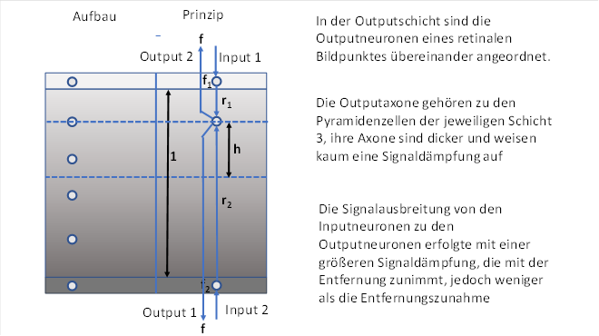
Figure 11: Brightness module

Symbolically represented are the two output neurons belonging to a pixel of the retina with signals inverse to each other. Exactly on the connecting line of the two input neurons, the output neurons are distributed at approximately the same distance.

Input and output neurons thus form a narrow eye dominance column.

Let f₁ be the firing rate of the light-on neuron and f₂ be the firing rate of the dark-on neuron.

We assume a brightness u and assign the following values to f₁ and f₂ . Let f₁  be the brightness of the light-on ganglion cell, f₂ that of the dark-on ganglion cell. We also refer to this ganglion cell as the light-off cell. We assume here that the dark-on submodality existed first. Therefore, it forms the lower of the two input layers in the thalamus and cortex.

Originally, each class 4 input layer had an associated class 3 output layer just above it - so both the submodalities and the neuron class layers divided and rearranged themselves for each submodality.

This resulted in the input layers 4-Hell-On and 4-Hell-Off and the layers two output layers 3-Hell-On and 3-Hell-Off.

However, since the light-on receptor was a descendant of the dark-on receptor, they were both signal-compatible, i.e. signal-related. Therefore, the output neurons of the lower output layer S3-Dark-On could also receive the excitation from the output neurons of the upper layer S4-Light-On. The input layer S4-Hell-On became superfluous and regressed in the course of evolution.

The excitation transmitted from the input neurons into the system should propagate through the layer and reach every neuron of the eye dominance column. The specified cable equation for markless axons applies here.

We consider a selected output neuron, which has the distance r₁ and r₂ from the input neurons. The excitations from both input neurons excite the output neuron according to the formula

As already shown on the Hessian matrix of the transfer function, there is a global maximum of the firing rate. We want to know where the output neuron with the strongest excitation is located for given firing rates f₁ and f₂ .

We determine the maximum by setting the derivative to zero.

We note that the distance between the two input neurons is equal to 1, the output neuron has distance h from the centre of the output layer.

Then applies:

This is exactly the equation we have already obtained for the colour module with vertical signal mixing. Therefore, the same results will be derived from it.

                                  (Main formula 1)

                                (Main formula 2)

               (Main formula 3)

 

This formula allows us to calculate from the firing rates f₁ and f₂ at which point h the output neuron has the maximum firing rate among all the others. Its output thus encodes the firing rate quotient. Instead of colours, this module can evaluate brightness. The formal apparatus is the same. A module can thus evaluate any modality as long as it decomposes into two submodalities, one of which is of the on-type and the other of the off-type.

Such a module is located in the Cortex just below the three-part colour module. We will call it the brightness module with vertical signal mixing.

Then the following statement applies:

The brightness module with vertical signal propagation in the visual cortex can recognise brightness as grey tones in the interval from white to black by characterising a maximum coded output with respect to the wavelength. It can detect brightness.

If the output of this brightness module leaves (up or down) and there is subsequently lateral neighbour inhibition between the output signals, the result is an output vector with sparse coding. Only those neurons remain active that are in the immediate vicinity of the excitation maximum. The excitation of the remaining neurons in the entire eye dominance column falls victim to lateral inhibition.

 

4.1.3.  New modalities in the vertical divergence module

 

The divergence modules with vertical signal mixing, vertical divergence modules for short, created new types of output. With each new neuron that could be created in the output layer, the new type of output was expanded by a new class of neurons that could do something that was not possible before: Detect colours, detect levels of brightness, detect mixtures of signals. This proved to be so significant and advantageous that each new class of neurons became an independent modality. This is how the modality colour, brightness, but also scent or taste came into being. The most important recognition feature of a new modality is its splitting in the neuronal system.

The independence of a new modality - the attainment of the modality property - had far-reaching consequences. Similar modalities (and submodalities, such as colour here) rearrange themselves. This means that the different colours began to separate in the brain. For example, if an eye dominance column for colour perception of a retinal pixel consisted of 20 output neurons running like a string of pearls from top to bottom through all three class 3 parvocellular cortex layers, the output of these 20 neurons divided into 20 new secondary brain areas. There were then 20 retinal images, but each of them was responsible for only one of the recognisable colours.

So if there was a green apple on the left and a red strawberry on the right, the apple image arrived in the retinal image that responded to green, while the red strawberry image appeared in a retinal image that responded to red and was in a completely different part of the cortex. It is somewhat like watching a colour film simultaneously on 20 different television sets, each of which displays only a spectral range encompassing one-twentieth of the visible colour spectrum. Therefore, we are justified in calling the output of this module colour modality. The term colour modality refers to the affiliation of neurons to this colour module, but equally to the output signals of this module.

It will be noticed that the mathematical apparatus is completely identical in colour vision and in brightness vision. Any other modality can also feed the signals of its receptors into such divergence grids. However, they should always be present as inverse signal classes. Then the strength of the primal magnitude can be derived from the position of the maximally excited neuron and the modality is amenable to fine analysis.

That is why there are on-signals and off-signals in many receptor systems. And where they were absent in one modality, the spinocerebellum and vestibulocerebellum could perform signal inversion. So for every motor signal in the cortex, there was an inverse signal in the cerebellum that also reached the cortex. This made it possible to analyse muscle strength, for example.

However, in order for a motor signal and the signal inverted from it in the cerebellum to arrive in the same half of the cortex, the motor signal had to change sides of the body before reaching the cerebellum, i.e. probably still in the spinal cord, before ascending to the cortex. So there had to be (for motor signals) a signal crossing at the spinal cord level that exclusively supplied the cortex, while the uncrossed signals reached the olive nucleus, so also moved to the other side and were inverted in the cerebellum. The ascending projection united the original signals and the signals obtained from them by inversion in the cerebellum in a common motor divergence module with vertical signal superposition. In this way, muscle strength, for example, could be finely dosed because it became measurable.

Extreme value coding takes place in the output layers of divergence modules. The maximally excited neuron evaluates the respective submodality with regard to its signal strength. Its activity evokes what neurologists and philosophers call qualia with regard to an elementary stimulus.

This reveals a fundamental problem of understanding. For physicists and many scientists, brightness is the energy content of the perceived light. For physicists and scientists, colour is the wavelength of light. Smell is the intensity ratio of substances that are present in the air through evaporation.

Neurologists, brain researchers and philosophers also discuss brightness, colour or smell. However, they do not mean the states of light energy, light wavelength or mixing ratio of scents in the air that exist outside our brain. They mean the mental state in the brain, which they call qualia and which seems to defy scientific explanation.

In this monograph, it is shown that brightness, colour, smell, muscle tension and many other things in a vertical divergence lattice lead to the specific maximum excitation of a neuron located at a mathematically defined level in the outpu layer of the respective submodality.

In those people whose outpu layer has the same thickness and the same number of neurons with regard to a submodality, as well as the same topological arrangement, exactly the same neurons are activated when a certain submodality, e.g. the colour of light, is analysed. These brain sections or brain layers could then (theoretically) be exchanged in different people without falsifying the analysis results.

In this respect, the primary cerebral cortices of the human cortex are constructed in the same way in different people and are in principle compatible with each other. However, if someone has an outpouch layer S3 in a primary cortex area that is significantly thicker than in most people, they can analyse the modality in question (colour, brightness, pitch, ...) somewhat more finely, and thus receive more intermediate levels during the analysis.

If an output layer S3 is missing, the person concerned is "blind" (insensitive) to the associated submodality (colour blindness, blindness, smell disorder, movement disorder, ...), but a failure of receptors can also cause this. It is particularly tragic when this is caused by congenital genetic defects, because those affected then never experience this perception throughout their lives. The lack of experience makes it particularly difficult to explain to those affected the existence of the submodality that is missing for them.

The brightness and colour modules with vertical signal superimposition significantly expanded their scope of analysis when a growth of the outpu layers occurred in the horizontal direction. The strong lateral expansion of the cortex layers could be recognised by the increase in size of the cortex and the wrinkling that occurred. If a layer is folded, it can have more surface area in the same space. Based on the development of the folds in the cortex layer, it can be concluded whether the animal in question is evolutionarily older (fewer folds, small size) or evolutionarily younger (more folds, larger area).

The principle of divergence grids with spatial signal superposition is first described using motor function as an example. All receptors that control motor function end in different sensory cortex layers. These form precisely the divergence modules that are described below.

The following section examines the consequences of lateral layer growth, pretending that thickness growth did not occur. This is out of touch with reality, but it is often useful to consider two different processes decoupled and on their own. Therefore, we now analyse the divergence lattice with lateral signal propagation and pretend that vertical signal propagation does not exist because the outpouch layer is a single-layer neuron layer.

Only then will the vertical and lateral layer growth in the cortex be analysed and the principle of cortical divergence modules with spatial signal propagation be dealt with. By taking this approach, I hope not to overwhelm those readers who will already have enough problems with the mathematical formula apparatus.